Blog
Cause-Effect Graphing: Notation, Process, and Examples

Abhilash
Published on

Table of contents
Lorem ipsum
Lorem ipsum
Lorem ipsum
Lorem ipsum
Lorem ipsum
Cause-effect graphing is a black-box test design technique that systematically derives test cases from specifications where multiple input conditions combine to produce specific outcomes. The problem it solves, namely testing rule-based business logic where several conditions interact, describes the substance of most modern enterprise applications, from permission systems to eligibility engines to pricing rules.
This page sets out the notation, the constraints, the full process, two complete worked examples, the relationship to neighbouring techniques, the common mistakes, the tooling, and the discipline that separates effective use from misuse.
What is Cause-Effect Graphing Actually?
Cause-effect graphing is a structured technique for converting a natural-language specification into a graph that captures the logical relationships between input conditions, called causes, and output behaviours, called effects, and then converting that graph into a set of test cases through a decision table.
Three components define the technique.
Causes are the input conditions or events the specification responds to, and each cause has a binary truth value, present or absent, true or false.
Effects are the output behaviours or system responses the specification produces, and each effect also has a binary value.
The graph is the directed structure that connects causes to effects through Boolean operators, namely identity, NOT, OR, and AND, along with constraints that exclude impossible combinations.
The technique produces test cases that exercise each unique combination of causes that produces a distinct effect, while excluding the combinations the constraints rule out as impossible. The result is a set of test cases that covers the rule-based logic of a specification without exhaustive enumeration of every possible input combination, which is the efficiency that makes the technique worth learning.
Cause-effect graphing sits inside the black-box testing toolkit alongside equivalence partitioning, boundary value analysis, and decision-table testing, and its specific contribution is to handle the case where multiple input conditions combine in non-trivial ways to produce different outputs. Where a single input maps to a single output, simpler techniques do the job with less effort, but where the logic branches on the interaction of several conditions, cause-effect graphing is the technique built for the shape of that problem.
Why the Technique Still Matters
It is fair to ask why a technique from 1973 belongs in a modern testing practice at all, and the honest answer is that its relevance rests on the nature of the problem rather than on the era it came from.
The applications that dominate enterprise software today are saturated with rule-based logic. A permission system decides what a user may see based on their role, their subscription tier, and the state of their account.
An eligibility engine decides whether an applicant qualifies based on age, income, residency, and history. A pricing engine decides what a customer pays based on volume, contract terms, region, and promotions in force. Each of these is a lattice of conditions combining to produce a discrete outcome, which is precisely the pattern cause-effect graphing was built to test.
The techniques that surround it in the black-box toolkit do not address this pattern. Equivalence partitioning tells you which values to pick for a single input, and boundary value analysis tells you where the dangerous edges of that input sit, but neither says anything about how several inputs interact to select an outcome.
Cause-effect graphing is the technique that reasons about the interaction, which is why it endures even as the surrounding practice has changed beyond recognition since it was first described.
The Notation, A Practitioner's Reference
The graph uses a small notation set, which is one of the reasons the technique is learnable in an afternoon even though applying it well takes practice.
Four functions link causes to effects, and five constraints restrict the combinations the graph permits.

The Four Functions
The functions describe how a cause or set of causes produces an effect, and together they are sufficient to express any Boolean relationship, with more complex logic built by composing them.
Identity: Effect e is true when cause c is true, and false when c is false. It is the simplest possible link, a direct pass-through from one condition to one outcome.
NOT: Effect e is true when cause c is false, and false when c is true. It is the negation of the identity relation, used when an outcome is triggered by the absence of a condition rather than its presence.
OR: Effect e is true when at least one of causes c1, c2, c3 is true. It is Boolean disjunction across multiple causes, used when any one of several conditions is enough to trigger the outcome.
AND: Effect e is true when all of causes c1, c2, c3 are true. It is Boolean conjunction across multiple causes, used when every condition must hold before the outcome occurs.
The reason four functions suffice is that any Boolean expression, however complex, can be rewritten as a composition of identity, negation, conjunction, and disjunction.
A rule such as "accept the claim when the policy is active and either the documentation is complete or a waiver is on file" decomposes into an AND over the policy condition and an OR over the documentation and waiver conditions, and the graph captures exactly that structure visually.
The Five Constraints
Constraints restrict the combinations of causes and effects the graph permits, and they exist to prevent test-case generation from producing combinations that cannot occur in the real system.
Skipping them is the single most common way the technique is misused, because a graph without constraints generates test cases for impossible situations, wasting execution time and producing failures that are not real defects.
Exclusive constraint (E): Either c1 or c2 can be true, but not both simultaneously. It is used between mutually exclusive causes, for example a payment that is either by card or by bank transfer but never both at once.
Inclusive constraint (I): At least one of c1, c2, c3 must be true, so it is not permitted for all of them to be false at the same time. It is used where the system requires at least one selection from a set.
One and Only One constraint (O): Exactly one of c1 or c2 must be true. It is stronger than the exclusive constraint because it also forbids both being false, used where the system demands precisely one choice, such as a required single-select field.
Requires constraint (R): If c1 is true, then c2 must also be true. The truth of c1 requires the truth of c2, used for dependency relationships, for example that an express-shipping flag can only be set if a delivery address is present.
Mask constraint (M): If effect e1 is true, then effect e2 is forced to false. Unlike the other four, this constraint operates between effects rather than causes, and it captures cases where one outcome suppresses another, such as a hard rejection suppressing any further processing message.
The five constraints handle the common cases of impossible combinations, and the practitioner skill that distinguishes real use of the technique from textbook use is specifying them accurately.
A team that draws the functions but skips the constraints produces a decision table full of columns for situations the system can never encounter, and the wasted effort of building and running those tests, plus the noise of their spurious failures, is exactly what the technique was supposed to eliminate.
The Process, From Specification to Test Cases
The technique follows a defined process, and five stages move a team from a written specification to an executable test set. Each stage has its own discipline, and the quality of the final test cases depends far more on the care taken in the early stages than on the mechanical conversion at the end.
1. Stage One, Decompose the Specification
Large specifications produce unworkably complex graphs, so the first stage breaks the specification into smaller pieces, each of which can be analysed independently. The decomposition typically follows the natural structure of the specification, meaning distinct features, distinct user flows, and distinct rule modules, and each piece is then handled as its own cause-effect graph.
The discipline of decomposition is to break the specification into pieces small enough that each graph stays workable, typically fewer than fifteen causes per graph, while keeping the pieces semantically coherent so that a single rule is not split awkwardly across two graphs.
A good decomposition respects the seams the specification already has, whereas a poor one cuts across a rule and loses the interactions that matter.
2. Stage Two, Identify Causes and Effects
The second stage examines the specification and extracts the distinct input conditions, the causes, and the output behaviours, the effects. Each cause and effect must be a binary proposition, capable of being true or false, present or absent, since the whole technique operates on Boolean values.
The discipline here is precision. A specification statement such as "the user submits a claim with valid documentation" contains multiple causes, namely that the user submits a claim, that documentation is attached, and that the documentation is valid, and each of these is a separate cause.
Conflating them into a single composite cause loses the analytical power of the technique, because the whole point is to discover how those conditions interact, and a composite condition hides the interaction inside itself.
The habit to build is to read every specification sentence suspiciously, asking whether it smuggles two or three conditions into one clause.
3. Stage Three, Construct the Graph
The third stage builds the graph itself. Causes are placed on the left, effects on the right, and the Boolean operators connect the causes to the effects according to the logical structure of the specification, with constraints added wherever the specification implies impossible combinations.
The graph is typically drawn by hand for small specifications and with graphing tools for larger ones, and the visual structure is not decoration, it is the mechanism that surfaces errors.
Seeing the causes and effects laid out with their connections makes gaps visible in a way that a paragraph of prose never does, and it is common for a practitioner to discover, only when drawing the graph, that the specification never actually says what happens when two particular conditions are both false.
4. Stage Four, Convert to a Decision Table
The fourth stage converts the graph into a limited-entry decision table. Each column of the table represents a unique combination of cause values that produces a distinct combination of effect values, and the table is constructed by systematically tracing through the graph, identifying the distinct rule sets, and recording the effects each produces.
The decision table is the formal test artefact, and each column becomes one test case. The graph was the analytical tool, and the table is the deliverable, which is a distinction worth holding onto because it explains why both steps exist rather than one.
5. Stage Five, Derive Test Cases
The fifth stage converts each column of the decision table into an executable test case. The test case specifies the inputs that satisfy the cause combination, the expected outputs that should match the effect combination, and the test data, preconditions, and assertions necessary to execute the test.
The test cases are then handed to the execution layer, automated where appropriate, and linked back to the requirement they verify, which closes the loop between the specification the analysis started from and the tests that now guard it.
Why the Graph and the Decision Table Both Exist
A practitioner question arises naturally, which is that if the deliverable is a decision table, why bother with the graph at all, and why not write the decision table directly. The answer is that the graph is an analytical tool, not merely an intermediate format, and its visual structure surfaces three classes of error that direct decision-table construction routinely misses.
The first is missing causes. A natural-language specification may imply a condition without stating it explicitly, and drawing the graph forces the practitioner to enumerate every condition that contributes to an effect, which catches the implicit ones that a hurried table would omit.
The second is missing effects. A specification often describes what happens in the common cases without enumerating the exception cases, and the graph structure makes those gaps visible, since an effect with no path leading to it, or a combination of causes with no effect attached, stands out visually.
The third is missing constraints. A specification may describe the permissible combinations without explicitly excluding the impossible ones, and drawing the graph forces the practitioner to consider every combination, which surfaces the cases the specification left implicit.
The graph is the thinking tool and the decision table is the deliverable, and skipping the graph is possible but sacrifices the analytical rigour the technique was built to provide.
A Worked Enterprise Example
Generic examples of light switches and vending machines have dominated the cause-effect graphing literature for decades, and they teach the mechanics while hiding what actually matters, which is how the technique behaves on real business logic. An enterprise-shaped example is more useful.
Consider a specialty insurance marketplace where brokers submit claims through a portal, and the specification governs whether a submitted claim is accepted into the underwriter queue, rejected, or returned to the broker for additional information.
The specification, in practitioner-readable form, reads as follows.
A broker submits a claim, and if the policy is active on the loss date and the claim falls within coverage limits and the required documentation is attached, the claim is accepted for underwriter review. If the policy is not active on the loss date, the claim is rejected with a policy issue. If the claim falls outside coverage limits, the claim is rejected with a coverage issue. If the required documentation is not attached, the claim is returned to the broker for additional information.
The causes are the input conditions the specification responds to.
C1, the broker submits a claim.
C2, the policy is active on the loss date.
C3, the claim falls within coverage limits.
C4, the required documentation is attached.
The effects are the discrete outcomes the specification produces.
E1, the claim is accepted for underwriter review.
E2, the claim is rejected with a policy issue.
E3, the claim is rejected with a coverage issue.
E4, the claim is returned for additional information.
The logical relationships connect the causes to the effects.
E1 is true when C1 AND C2 AND C3 AND C4.
E2 is true when C1 AND NOT C2.
E3 is true when C1 AND C2 AND NOT C3.
E4 is true when C1 AND C2 AND C3 AND NOT C4.
The constraints capture what the specification implies but does not state outright. The four effects are mutually exclusive, since a single submission cannot produce more than one outcome, which is a mask relationship among the effects. And C1 is a prerequisite for any effect, since with no submission there is no outcome to test at all, which is a requires relationship.
Reading the Graph
Before the table, it helps to picture the graph, since the visual is the part most readers have never actually seen.
On the left sit the four causes as nodes, stacked C1 through C4. On the right sit the four effects, E1 through E4. From the causes, edges run rightward through Boolean operators to the effects.
E1 is fed by an AND node gathering all four causes, with C2, C3, and C4 entering directly and the whole conjunction gated by C1. E2 is fed by an AND node combining C1 with a NOT node on C2, so the edge from C2 passes through a negation before reaching the operator. E3 combines C1, C2, and a NOT on C3. E4 combines C1, C2, C3, and a NOT on C4.
Over on the effect side, a mask constraint links the four effects so that whenever one is true the others are forced false, and a requires marker ties every effect back to C1. Drawing it this way makes the precedence obvious, since the eye follows C1 as the gate that everything else depends on, and it makes the symmetry of the three rejection paths visible in a way the prose does not.
The Decision Table
Tracing the graph produces the following limited-entry decision table, where each column is a distinct rule and a dash indicates that the value of that cause does not affect the outcome, because an earlier cause in the precedence has already determined the effect.
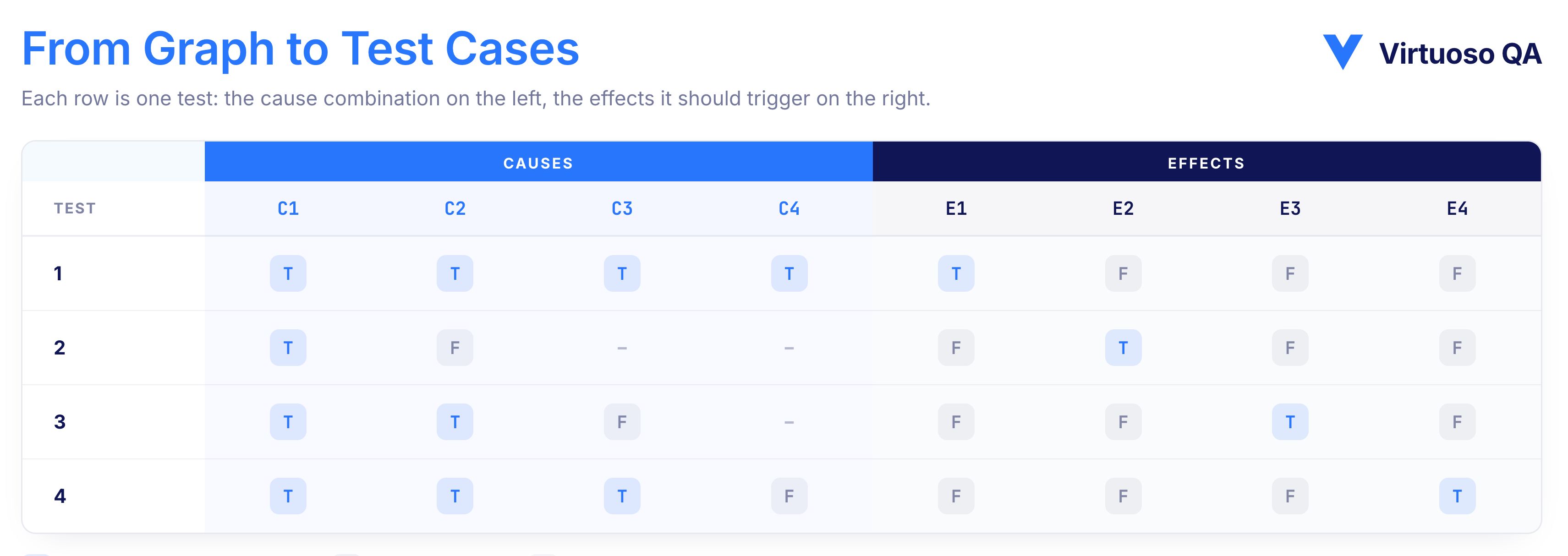
The four columns produce four executable test cases. The dashes carry real meaning, since in test 2, once the policy is inactive, the coverage and documentation conditions no longer change the outcome, because the claim is rejected on the policy issue regardless, so there is no need to enumerate their values.
The number of test cases is dramatically smaller than the full Cartesian product of the cause values, which would be two to the power of four, or sixteen combinations, because the logical structure rules out the combinations that produce no observable behavioural difference.
The four test cases cover the four distinct behavioural outcomes the specification describes, and adding more test cases beyond these four produces no additional defect-detection power, because every additional input combination would fall into one of the four buckets already covered. That collapse from sixteen to four is the technique earning its keep, and on a larger specification with eight or ten causes the collapse is far more dramatic, turning hundreds of theoretical combinations into a handful of meaningful tests.
How the Test-Case Count Collapses
It is worth dwelling on why the technique produces so few test cases, since the reduction is the whole economic argument for using it.
A specification with n independent binary causes has two to the power of n possible input combinations, which grows explosively, so ten causes yield 1,024 combinations and twenty causes yield over a million. Testing all of them is infeasible, and testing a random subset is unprincipled.
Cause-effect graphing collapses the count in two ways.
First, the logical structure means many combinations produce the same effect, so once a combination has been tested for a given effect, other combinations that produce the same effect add nothing, and they are folded together.
Second, the constraints eliminate combinations that cannot occur at all, removing whole branches of the theoretical space as impossible. What remains is one representative test case per distinct behavioural outcome, which is the minimum set that still exercises every rule the specification contains.
The technique is, in effect, a principled way of finding that minimum set by reasoning about the logic rather than by sampling the inputs, and that is why it detects the interaction defects that random or single-variable testing miss.
When Cause-Effect Graphing is the Right Choice
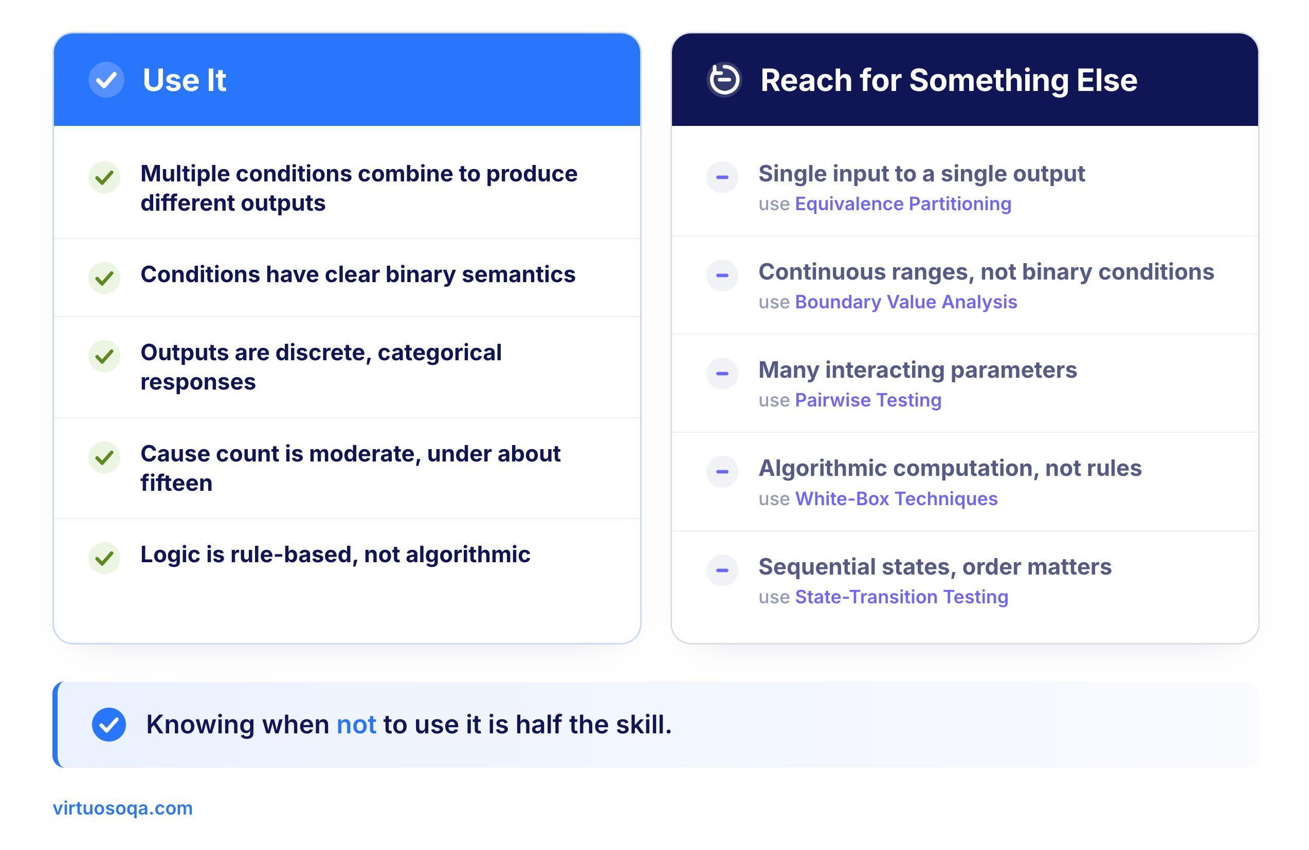
The technique is powerful when applied to the problems it was built for and weak when applied to others, and five conditions favour it.
The Specification Involves Multiple Input Conditions Combining to Produce Different Outputs
Eligibility rules, pricing engines, permission systems, workflow gates, and compliance checks all fit this pattern, whereas a single input producing a single output is better served by simpler techniques.
The Conditions Have Clear Binary Semantics
Cause-effect graphing operates on Boolean truth values, so continuous parameters require discretisation before the technique applies, which adds analytical work and may not preserve all the relevant behaviour.
The Outputs Are Discrete Categorical Responses Rather Than Continuous Values
The technique is most natural where the system produces a small set of distinct outcomes, and systems producing continuous numeric output are better probed by techniques that explore the output space directly.
The Number of Causes is Moderate
The graph stays workable up to roughly fifteen to twenty causes, beyond which the visual structure becomes unwieldy and the specification should be decomposed further or handled with pairwise generation for combinatorial coverage.
The Logic is Rule-Based Rather Than Algorithmic
The technique handles "if these conditions, then this outcome" specifications well and "compute this from these inputs" specifications poorly, because it presumes a structural relationship between conditions and outcomes rather than a computational one.
When it is Not the Right Choice
The same five conditions inverted indicate when to reach for a different technique, and naming them plainly keeps a team from over-applying the method.
Simple single-input, single-output relationships are better served by boundary value analysis and equivalence partitioning.
Continuous parameters are better served by techniques that handle ranges directly.
High-parameter spaces beyond about twenty causes are better served by pairwise or combinatorial generation.
Algorithmic computations are better served by white-box techniques that follow the code paths.
Sequential workflows, where the order of events matters and the system moves between states, are better served by state-transition testing.
The discipline is matching the technique to the shape of the problem. A team that defaults to cause-effect graphing for every test design produces over-engineered analyses for simple problems and falls short on problems the technique was never built for, and knowing when not to use it is as much a mark of competence as knowing how to use it.
How it Relates to the Other Black-Box Techniques
Cause-effect graphing is not a rival to the other black-box techniques but a complement, and a complete test design usually draws on several at once.
Each neighbouring technique decides something different, and each fits alongside cause-effect graphing in its own way.
Equivalence partitioning decides which value classes exist for a single input, which means it chooses the actual values that stand behind each binary cause in the graph.
Where cause-effect graphing treats "the policy is active" as a true-or-false condition, equivalence partitioning is what tells you which concrete inputs make that condition true or false.
Boundary value analysis decides the dangerous values at the edges of a range, so it picks the specific edge values for any cause derived from a range. If a cause is "the claim falls within coverage limits," boundary analysis is what probes the exact limit where that condition flips.
Decision table testing decides the mapping of condition combinations to outcomes, and it is the deliverable that cause-effect graphing produces, with the graph as the analytical step that comes before it. The two are stages of one method rather than separate techniques.
State transition testing decides behaviour across states and the events that change them, which means it handles the sequential, stateful logic that cause-effect graphing does not model. Where the order of events matters and the system moves between states, state transition testing takes over.
Equivalence partitioning and boundary value analysis decide the concrete values that make a cause true or false, cause-effect graphing decides how those causes combine to select an outcome, and decision table testing is the tabular form that combination takes. On a rule-heavy feature, a thorough tester uses all of them together.
Common Mistakes in Cause-Effect Graphing
A handful of recurring mistakes account for most of the cases where the technique disappoints, and naming them is the fastest route to using it well.
1. Skipping the Constraints
The most common and most damaging mistake, since a graph without constraints generates test cases for combinations the system cannot encounter, wasting effort and producing failures that are not real defects.
1. Conflating Composite Conditions
Treating "submits a valid claim with documentation" as one cause rather than three hides the very interactions the technique exists to expose, and it is the mistake that most quietly undermines the analysis.
3. Letting the Graph Grow Too Large
A graph with thirty causes is not a tool, it is a liability, and the fix is decomposition into coherent smaller graphs rather than heroic effort on one enormous diagram.
4. Skipping the Graph and Writing the Table Directly
Faster in the moment, but it sacrifices the error-catching that the visual structure provides, so the missing causes, effects, and constraints that the graph would have surfaced slip through instead.
5. Failing to Trace Back to Requirements
A test case that is not linked to the requirement it verifies loses its meaning the moment the specification changes, and the discipline of maintaining that link is what keeps the test set honest over time.
6. Applying the Technique to the Wrong Problem Shape
Using it on continuous parameters, algorithmic computation, or sequential workflows produces awkward analyses that would have been cleaner with the right technique.
Cause-Effect Graphing in the AI-Coded Era
A new dynamic has raised the value of cause-effect graphing, because it turns a test-design technique into a code-review technique as well.
AI coding assistants now draft eligibility rules, permission checks, workflow gates, and pricing decisions before human review, and the generated code looks plausible while frequently missing the interaction between conditions in ways that surface only in production.
Cause-effect graphing catches exactly these errors, because it forces the team to enumerate every condition, effect, and combination, surfacing gaps that pure unit testing does not. It also exposes the reverse problem, where AI invents constraints and special cases the specification never asked for, since analysing the graph against the original specification reveals the divergence. The access-control override earlier is precisely the kind of logic an assistant gets subtly wrong.
The pragmatic posture is to apply the technique to AI-generated business logic before it reaches the test suite, so it does double duty as both a test-design tool and a review tool.
Where Virtuoso QA Fits
Virtuoso QA supports the workflow downstream of the graph, taking the analytical output of cause-effect graphing and turning it into continuous verification.
Readable test cases from the decision table: The decision table derived from the graph translates into Natural Language Programming test cases that read in the language of the specification, so the rule a test verifies is legible to the analysts and reviewers who care about it, not only to engineers.
Traceability by default: Each test case carries its link to the requirement, use case, and journey it inhabits, which preserves exactly the specification-to-test connection the fifth stage of the process depends on.
Resilient execution: Tests execute across the cross-browser execution grid, with self-healing absorbing the minor interface changes that would otherwise break rule-based tests on every commit, so the cases you derived once keep verifying the rule as the application evolves.
Accelerated derivation: Agentic test generation can produce draft cause-effect-aligned test cases from existing specifications, requirements, and use cases, which shortens the test-case derivation step without removing the analytical judgement that decides which cases matter.
Failure diagnosis.: AI Root Cause Analysis identifies whether a failure is a defect in the rule the test verifies, a defect in the related logic the rule interacts with, or a flake unrelated to the underlying behaviour, which is the distinction a rule-based test most needs when it goes red.
The combination applies continuous verification to rule-based business logic, where the analytical rigour of cause-effect graphing produces the test cases and the verification fabric executes them and surfaces the failures. The technique supplies the thinking, and the platform supplies the endurance.
Frequently Asked Questions
What are the Notations Used in Cause-Effect Graphing?
What is the Difference Between Cause-Effect Graphing and Decision-Table Testing?
When Should Cause-Effect Graphing Be Used?
What is a Cause in Cause-Effect Graphing?
What is an Effect in Cause-Effect Graphing?
How Does AI-Assisted Coding Affect Cause-Effect Graphing?